Last Updated on January 23, 2026 by Maged kamel
Maximum deflection distance for a simply supported beam under a triangular load-Numerically.
We want to determine the maximum deflection distance for a triangular load acting on a simply supported beam 6.0 m long. The maximum load intensity is 2.0 kN/m. Our task is to find the x-max distance using the Numerical method. We will solve this by using the Newton-Raphson method for roof findings.
The three equations for the change of slope & slope, and deflection values.
This is a list of three items: the first is the change-of-curvature equation, and the diagram shape for a supported beam under a triangular load, where w0 is the maximum value of the triangular load, and x is the distance for which we want to calculate the change of curvature.
The second item is the curvature slope equation, and the diagram shape for a supported beam under a triangular load, where P is the maximum value of the triangular load, and x is the distance for which we want to calculate the curvature slope.
The third item is the slope of the curvature equation and the diagram shape for a supported beam under a triangular load, where w0 is the maximum value of the triangular loa,d and x is the distance for which we want to calculate the deflection.

The next slide image shows the slope and deflection equations of a simply supported beam under a uniformly Triangularly distributed load.
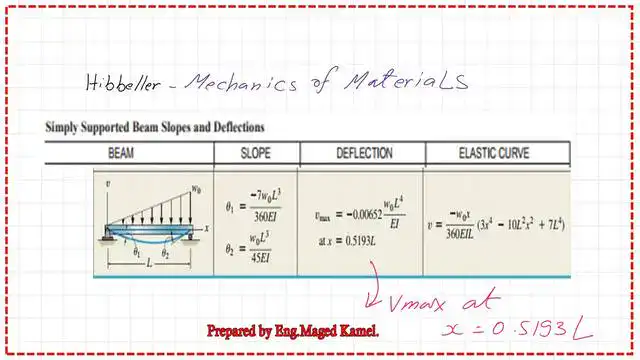
Estimating the maximum deflection distance from the left support x max is required. The point of the maximum deflection is the point at which the slope of curvature is zero. Usually, we use the Newton-Raphson method we want to get the point where Y value =0.
The function value f(x) was in the numerator. Refer to the relation, where X0 is the starting point, f(x0) is the function value at x0, and f'(x0) is the function’s slope value at point X0.
The revised Newton-Raphson equation is based on the slope equation.
To use the Newton-Raphson equation, we will work with the y’ curve, since it changes from positive to negative. A root point for zero slopes will give us the point of maximum deflection. Instead of dealing with the y curve as in the case of the original form of the Newton-Raphson equation, we are now dealing with the y’ function.

The steps for estimating x max using the analytical solution.
The modified equation for the root point will be as, for the first point after setting an initial point of, which will be given a value of 2.00m, less than the L/2.
Our first trial value of x0 is =2.00m.
We need f'(2) and f”(2) to apply it in the adjusted equation. We have the expression for F'(x) for the slope value of the curve due to the triangular load, and also y”, the change of curvature of the beam. We plug in with x0=2.0m and get the two values of f'(2) and f”(2), as shown in the next slide. We need to use 1/EI=1/8*10^4.

Our second trial value of x0.
Then we plug in x0 as a second trial = 3.30 m, and we get the second maximum deflection distance of 3.1169 m. Our third x0, with a starting value of 3.1169 m, yields a maximum deflection distance of 3.1169 m.


Then we plug in x0 as a second trial (X2 = 3.1169 m) and obtain the third maximum deflection distance of 3.116 m.
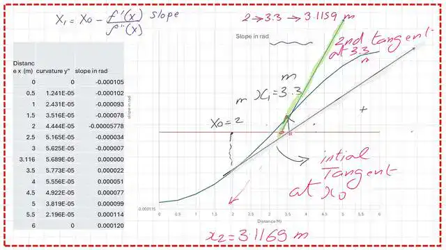
The following table shows the result of x0 when we start with an initial point of 2.0m for four iterations.

This is a graph of the slope. We start at x0 = 2 m and end up at x1 = 3.30 m. Please refer to the previous table.
In case our first trial value of x0 is =3.00m.
If somebody wishes to choose a starting point of 3.00 m. x0 with a starting value of 3.0m will lead us to a modified value of 3.1166m, as the maximum deflection distance.
Then, we plug in x0 as a second trial value of 3.1166 m and obtain the second maximum deflection distance of 3.116 m.
The following table shows the result of x0 when we start with an initial point of 3.0m for four iterations.
If somebody wishes to choose a starting point as=4.0. The x0 with a starting value of 4.00m will lead us to a modified value of 3.116m, as the maximum deflection distance.

The Modified Newton-Raphson equation.
We can use the modified Newton-Raphson Equation to determine the point of maximum deflection, but we will consider the following terms: f(x) from the slope equation, F'(x) from the curvature slope, F”(x) from the shear equation, and Q(x). The following slide contains a reminder of the equations needed to obtain the values for load, shear, and moment. We use the discontinuity function expressions.

We need to estimate the values of shear and moment for a starting point x0=2.00m, as we can see the Q(x0=2)=1.66 Kn while the value of M(X) for x0=2.0 m equals 3.555 KN · m.

We will obtain the slope at X0 = 2.0 m, which will be our f(x) in the expression for the modified Newton-Raphson method. The value of EIV dash or the slope equals-4.662 KN.m2. We plug the Modified Newton-Raphson equation into the equation and get x1 = 2.8739 m. Please refer to the following slide for more details

The following slide shows the details of estimating the different values of Xi using a starting point of X0 = 2.00 m. Thanks a lot.

You can review or download the PDf file used for this post from the following documents.
This is a link to the previous post, where I included a solved problem demonstrating the application of the Newton-Raphson equations for structural analysis.-structural analysis numerically by the Newton-Raphson method.
This is a good external reference. Holistic numerical method.
This is a useful link for a numerical analysis calculator.