5- What is the Linear Approximation method?

Last Updated on September 23, 2026 by Maged kamel

What is the Linear Approximation method?

What is Linear approximation?

Linear approximation, or linearization, is a method for approximating a function’s Value at a given Point. Linear approximation is useful because it can be difficult to find a function’s Value at a particular Point.

We have a function like that. We know the Value of x at a Point, which we call a. We know xa, the x-distance, and we know the coordinate Value, f(x=a).

Suppose we have another point that is considered close to point A. We can assume that we have a line tangent to that curve at Point a.

We can treat the function as linear at any point; we get the y-value from that line.

The linear approximation equation.

So the linear approximation is y = the Value of any point we need, starting from a given point xa and its Value f(a). We make this line with slope, then go to another point, say c. We get the Value of xc by substituting. We get the function Value of x_c. 

Linear approximation is a method for finding the y-value of point b, given the x-value of another point, a, and its y-value. The linear approximation Value L(x=xb) equals the function Value at a+( the slope of the tangent) *the difference between(the new Point x_b – the old Point x_a).

Solved problem #1: Find the linear approximation of y as f(x)=sin(x) at x0=0.

Our solved problem: Find the linear approximation of y as f(x)=sin(x) at x0=0. We write the equation in general form as: L(x)= approximately=f(a)+f'(a) *(x- a), where a is the starting point for which we know the Value of y as well as the f’ Value.

To develop L(x) for f(x)=sin(x), we get the f'(x) Expression, which is cos(x); the f(x) Value at x0=0 will be equal to=0, while f ‘ (0)=cos(0)=1. We consider (xb-x0)=x, the formula L(x)=0+(x-0)*1=X.

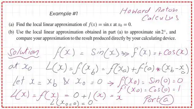
For part b, we need the local linear approximation of the function at x = 2; dx = 2e^x. L(2) = 2 degrees; we convert that to rad and get 0.0349066. The exact Value of f(x=2)= sin(2)=0.0348995. Please refer to the following slide for more details.

The following graph shows f(x), which is sin(x), and the line L(x) that passes through x0=0.

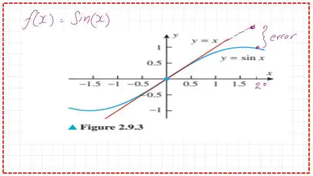
To estimate the PoPointalue of the error, we subtract L(x) from the actual Value. For solved problem #1, we get 7.6*10^-6.

Solved problem#2: find the linear approximation of y as f(x)=x^2 at 2.50.

As an application, we can obtain a linear approximation of any function and find the power, square root, or cube root of a number.

Our solved problem: find the linear approximation of y as f(x)=x^2 at 2.50. We put the equation in the general form by writing. L(x)= approximately=f(a)+f'(a) *(x- a, where a is the starting point for which we know the Value of y as well as the f’ Value.

Our next question is: Which Point is nearest to 2.50? The nearest Point to 2.50 is 2, for which we can get the Value of y, as well as the Value of the slope. Point 1: We Estimatee function Value at the starting Point a, which is equ0)^2= ^2 = 4.00- We need to estimate the slope Val;e, the x^2 to be differentiated is y’ = 2x
3- Get the Value of y’ at x=2, it will be=2*(2)=4.0.

4-We can apply the Expression and get L(x=2.50) =f(2.0)+(y’*(x_b-x_a), where a is the starting Point where x=2.0, while xb is the Point for which we want to approximate the Y Value, which is equal to 2.50.
5-The value of L(x=2.50)=4+((2)Point(2.50-2.0))=6.00.
6-The exact value= the approximated Value + error, apply in the equation of y=x^2, the exact Value is (2.50)^2=6.25, the approximated value=6.00. 7- The error value=6.25-6.0=0.25.

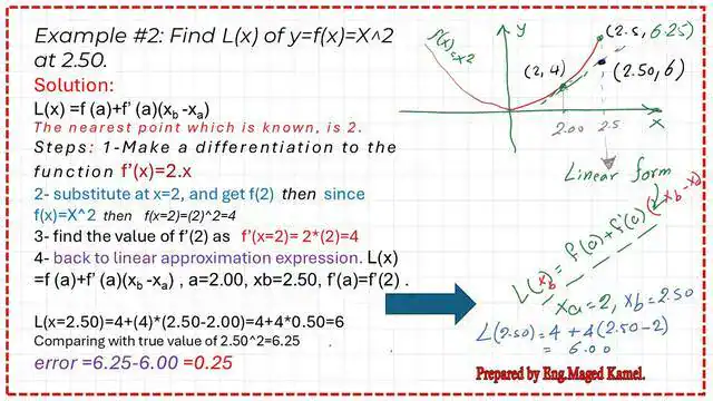
The following graph shows f(x) = x^2 and the line L(x) that passes through the x0 = 2 point.

You can review and download the data for this Post and the following Posts in the document below.

The next Post covers practice problems with linear approximation.

Here is a useful Link to the Linear approximation calculator- eMath Help.