
Last Updated on September 15, 2026 by Maged kamel
Upper bounds and Lower bounds.
A new subject to discuss is upper and lower bounds and the uniqueness theorem.
In our previous post, we had a Beam fixed at one end at support A and a roller support at point B, with a Load acting at point C at mid-span. The Load Value is 32λ, where λ is the collapse Load divided by the working Load. We want to estimate λ to find the Value of Pp for a Beam with a length of 1.0 m.
We can find λ using statics.
We have two hinges at the collapse, one at joint A and the other at joint C. Suppose we consider the Beam in the sketch, with a Load of 32*λ. We can estimate the reactions at A and C by taking moments about A and B. By = 16λ- 9, while Ay = 16λ + 9. Please refer to the following slide.
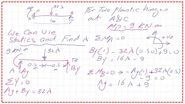
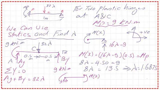
We verify the lambda Value by taking moments about point C on the right side; we have M(x) = Mp = (16λ – 9) * 0.50 = Mp. After simplifying, we get 8λ = 13.50, which implies λ = 1.6875.
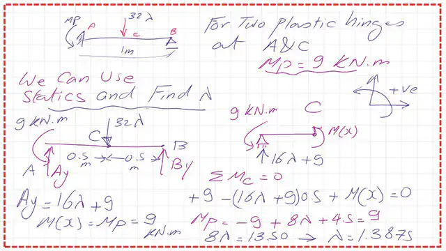
We verify the lambda Value by taking the Moment about point C on the left side: M(x) = Mp = – (16λ + 9) * 0.50 + 9 = Mp. After simplifying, we get 8λ = 13.50, which implies that λ = 1.6875.
The uniqueness theorem & lower and Upper bound theorems.
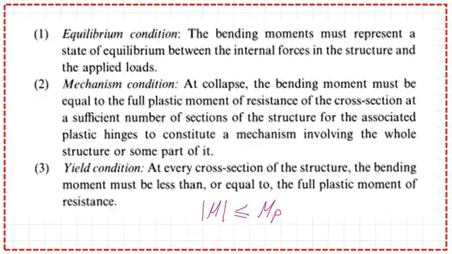
The uniqueness theorem has three requirements and guides the development of the true hinge locations and the nominal load estimate. The first point is equilibrium, which requires the same Mp value at the same point from the left and right sides.
The second point is the mechanism, where we make the system unstable by increasing the number of indeterminacies by 1. The yield is the bending Moment, which must be fp, the biggest Value in the diagram.
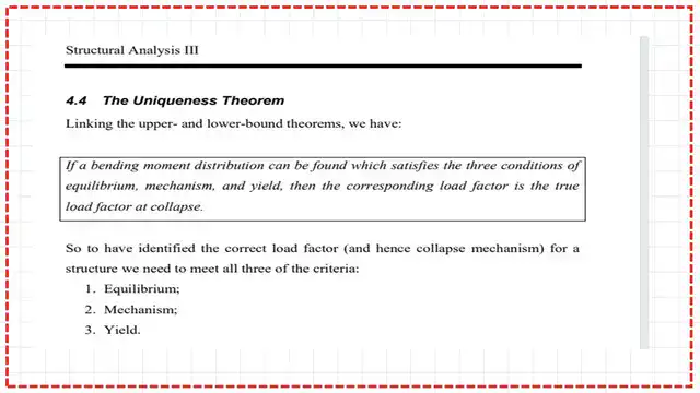
It has three equilibrium conditions and the mechanism conditions.
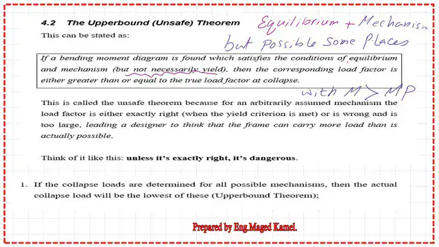
In the virtual work method, we assume a point at which the external and internal work are equal. At that point, we assume it is our chosen point, but someone else may select a different point and obtain a different Value of λ for this method under the upper bound theorem.
I quote: if a bending Moment diagram is found that satisfies equilibrium and the mechanism (but not necessarily yields), then “yield” means we could obtain a Value higher than the plastic Moment.
The corresponding Load factor is greater than or equal to the true Load factor at collapse. A question is: which point is correct and gives the exact Value of Mp?
This method is called the unsafe theorem because, for an arbitrarily assumed mechanism, the Load factor is either exactly right or exactly wrong; hence, it is called the upper-bound method. If the ccollapseloads are determined for all possible mechanisms, then the actual collapse Load is the lowest of these (upper bound theorem). For the static Load method, select the point that yields the highest Mp Value.
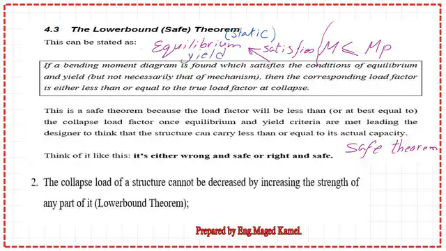
The Lower Bound Theorem satisfies two conditions: equilibrium and yield, but not necessarily the mechanism.
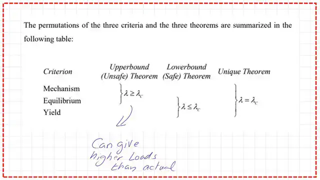
The collapse Load factor is related to the three theorems.
A practice problem for lower-bound points on the graph.
I will introduce a practice problem for the lower-bound discussion on the last slide. If we ha e a propped cantilever of length 10m and the plastic Moment is 266.667 kN·m, to find a point on the lower portion of the graph, we assume a nominal Load of 80 kN. We use t e static (equilibrium) method by superimposing the two bending-moment graphs. The MMa Value for P = 80 kN is -150 kN·m, while Pl/4 = 200 kN ·m. We find that both Ma and Mc are lower than the required Mp so that no collapse will occur.
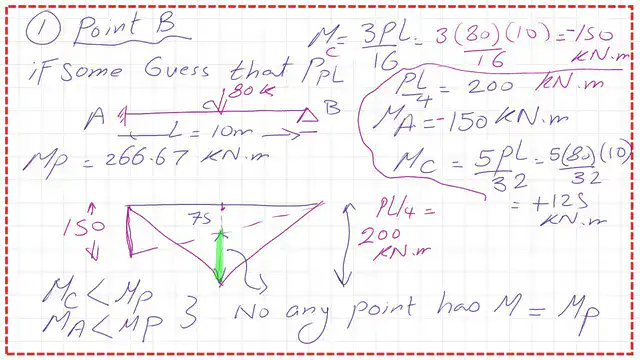
We assume the nominal Load is 120 kN. We use t e static (equilibrium) method by superimposing the two bending-moment graphs. The MMa Value for P = 120 kN is -225 kN·m, while PL/4 = 300 kN·m. We will find that both Ma and Mc have a lower Value than Mp; this is not the correct solution.

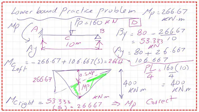
We assume the nominal Load is 160 kN. We use t e static (equilibrium) method by superimposing the two bending-moment graphs. The MMa Value for P = 160 kN is -266.67 kN·m, while PL/4 = 400 k ·m. We will find that both Ma and Mc have the same Value as Mp; this is the correct solution.
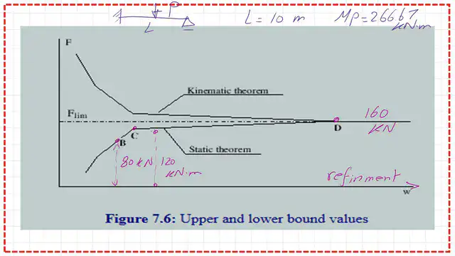
The graph shows the relation between the lower and upper bounds.
Next, we show the graph illustrating the differences between the lower and upper bounds when the Load or Moment is Pp or Mp. This horizontal line is the bound, or the actual Load represented by F at collapse.
The kinematic method yields values at least as large as the actual plastic Load.
We can represent the three points B, C, and D obtained from the practice problem. The bound is the actual Value, the kinematic theorem is the upper bound of collapse, and the static theorem gives a lower bound at points B and C, or matches the graph at point D.
Thanks a lot. You can view or download the PDF data from the next button.
For useful information on Structural Analysis III, most of the data used in this Post is quoted from the paper Structural Analysis-III.
The next Post continues the introduction to the lower bound and uniqueness.
Here is the Link to Chapter 8, Bending Members, in A Beginner’s Guide to the Steel Construction Manual, 14th ed.
Here is the Link to Chapter 8, Bending Members, in A Beginner’s Guide to the Steel Construction Manual, 15th ed.
Here is the Link to Chapter 8, Bending Members, in A Beginner’s Guide to the Steel Construction Manual, 16th ed.