
Last Updated on September 2, 2026 by Maged kamel
Matrix operations-part-1, orthogonal matrix, addition, and subtraction.
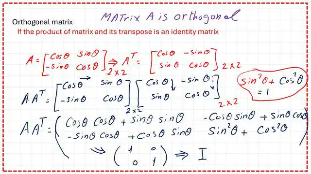
What is an orthogonal matrix?
Orthogonal means perpendicular. An example of two orthogonal matrices is given for the value of matrix A and its transpose. For a given matrix A, written as ( cos θ sinθ, -sinθ cosθ), its transpose can be formed by changing the rows into columns; the transpose will be ( cos θ -sinθ, sinθ cosθ). When we multiply both matrices, we get an identity matrix. Please refer to post 2 to learn about the transpose of a matrix.
When are two matrices said to be equal? If we have, for instance, matrix B and matrix C, then matrix B equals matrix C if each element of matrix B equals each element of matrix C, and both matrices should have the same dimension. For a given matrix A, if the value of a11=a, then the corresponding b11=3.
If both matrices B and C are (2×3), then matrix B equals matrix C. If a11=b11=3, also a12=-2=b12, which is x. When a11=b11=3, and also when a13=b=b13=-4, also if a22=c = b22 =-1, if c=-1.
There is an example of two matrices with the same dimensions that are not equal.
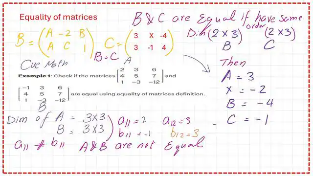
For these conditions, matrix B and matrix C are equal, or there will be equality between the two matrices.
Matrix operations-part-1.
Matrix addition & subtraction.
What are matrix operations? Adding matrices is the first operation in part 1 of matrix operations.
The first operation is adding two matrices or subtracting one from the other. For example, we have matrix A (2×3) as shown) and another matrix B.
Both matrices must be (2×3). Then, we can add these two matrices. A+B is the new matrix from addition, and each element is determined by adding similar elements in matrix A and matrix B.
The first row of the first column, a11 + b11 = 1 + 1 = 2, will be the new (A + B) matrix’s first row. Similarly, a21+b21=2+1=3 will be the new element in the second row and first column.
The final matrix is obtained by adding A and B. For the value of the second row with the third column =(4+(-4)=0. The dimension of matrix (A+B) must be (2×3).
While subtracting matrix B from matrix A is the same as for the process of addition except that we add A+( -1*B) as if we multiplied matrix B by (-1),thenู (-1) the new elements of (-B) will be as(-1*1,+2*-1,1*-1, 1*-1, 3*-1, -4*-1).
We add to the corresponding elements in matrix A. The final form of (A-B) is shown.
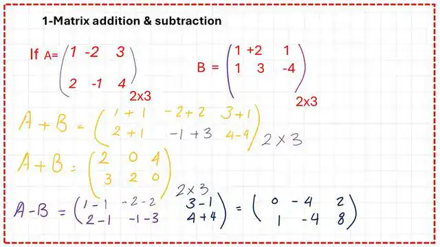
As (0,-4,2,1,-4, 8). Here is a list of the operations that can be done for matrices. The first item is adding A+B, which will be=B+A.
If we have three matrices, A, B, and C, we will add them all. Adding A+(B+C) will give the same result as adding (A+B)+(C). Adding A + (-A) = 0 is logical, since all elements are zeros. Adding A+0 will give matrix=A.
Scalar multiplication.
Scalar multiplication is the second operation of matrix operations part-1. It involves multiplying matrix A by a constant; the resulting matrix will be a multiple of that constant. For the shown 3×3 matrix, we want to multiply by 2.
The new matrix will have each element multiplied by 2, or twice the old matrix before multiplying.

Matrix multiplication.
Another operation is Matrix multiplication, the third operation in the matrix operations part 1.
We draw an arrow from left to right and another from top to bottom. We must ensure that the number of columns in the first matrix equals the number of rows in the other matrix.
We are multiplying a matrix of dimension (1×3) by another matrix of dimension (3×1). 1×3 means one row with three columns; 3 is common. The first three are the column numbers, and the others are the row numbers.
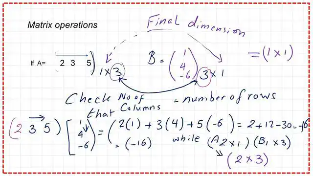
The dimension of the final matrix will be( 1×1), which is the product of the first element of matrix A by the last column dimension in the other matrix.
The final matrix dimension is (1×1), i.e., a single element. The final number equals (2*1 + 3*4 + 5*-6), which adds up to 16. The new matrix dimension will be(1×1).
You can view or download the PDF file for the first three posts from the following documents.
For a useful external link on types of matrices, visit Math is Fun.
This is a link to the next post, Matrix operations part -2.