blog posts

38a-Solved Problem 10-1-Design of Steel Continuous Beam-2-4.

September 15, 2026April 2, 2025 by Maged kamel

Brief description -post 38a -steel beam-Part 2/4 of solved problem 10.1.

Design of steel continuous beam-2-4 using Plastic theory, the upper bound theorem is used to get the required w -section for a continuous beam.

20-AISC Tables 9-3a, 9- 3 b, and C for Block shear-coped Beam.

September 13, 2026March 17, 2025 by Maged kamel

Brief data for post -20- Solved problem for coped beam using tables.

AISC Tables 9-3a,b, and C for the block shear-coped beam. Table 9-3a is for Tensile rupture. Table 9-3b is for Shear yielding and 9-3c is for Shear rupture.

38- Solved Problem 10-1- Design of Steel Continuous Beam-1-4.

September 15, 2026March 1, 2025 by Maged kamel

Brief description -post 38 -steel beam-Part 1/4 of solved problem 10.1.

solved problem-10-1 using Plastic theory, the upper bound theorem is used to get the required w -section for a continuous beam.

10-Two solved problems for a 3×3 Matrix using Crout’s LU option 1.

October 21, 2026November 1, 2024 by Maged kamel

Two solved problems for the Crout's LU decomposition.

Two solved problems for 3×3 matrix by Crout’s LU decomposition. Option 1 is used for which the matrix is converted to a lower matrix.

9A- A Second Option for Crout’s LU Decomposition- 3×3 Matrix

October 19, 2026October 29, 2024 by Maged kamel

LU decomposition for the Crout's method for 3x3 matrix-option 2

A Second option for Crout’s LU decomposition-3×3 matrix. How to covert the A matrix to an upper matrix? How to get the values of L and U matrices?

9d-Practice problem 5-5-8-Compute Mn.

September 13, 2026August 9, 2024 by Maged kamel

Brief description of the content of post 9d-Find nominal Flexure strength.

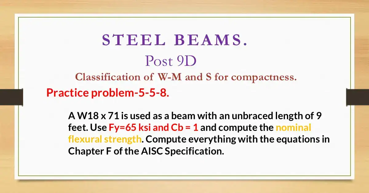
Practice problem 5-5-8 A W18 x 71 is used as a beam with an unbraced length of 9 feet. Use Fy=65 ksi and Cb = 1 and compute the nominal flexural strength.

9c-Practice problem 5-5-6-Compute Lp and Lr and φb*Mn.

September 13, 2026August 9, 2024 by Maged kamel

Brief description of the content of post 9c-solved problem 5-5-6.

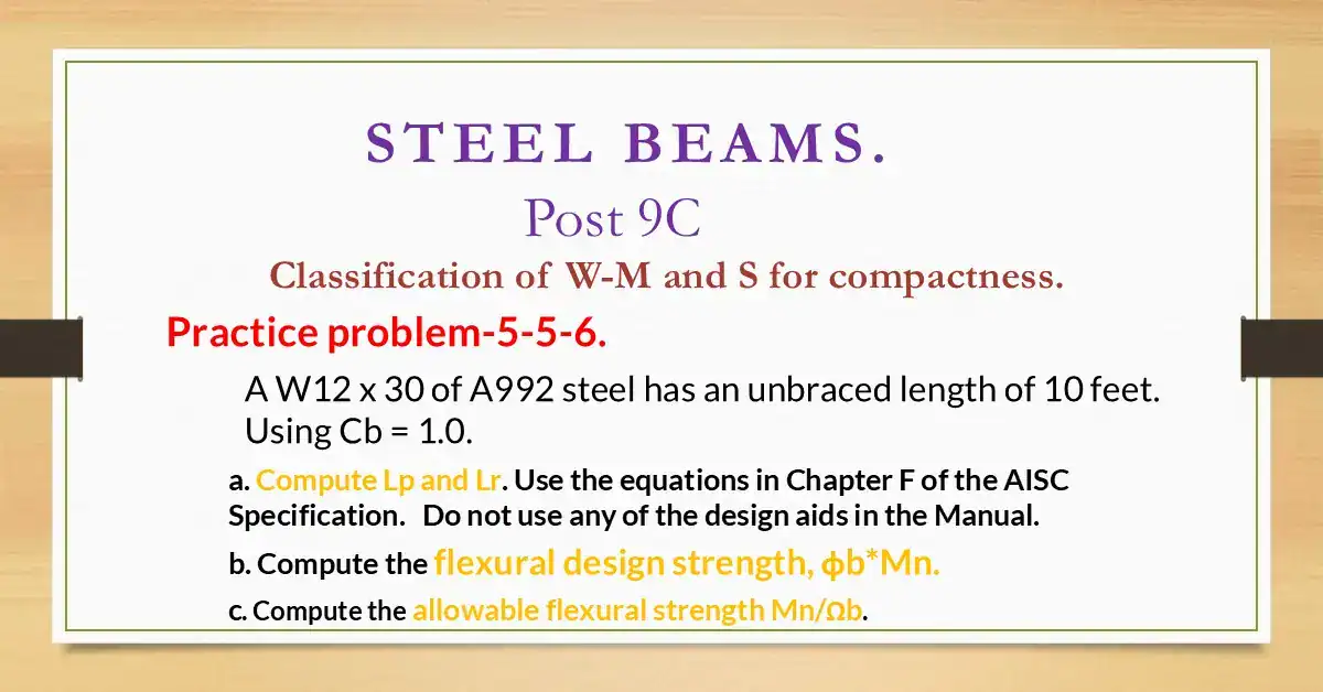
Practice problem 5-5-6 A W12 x 30 of A992 steel has an unbraced length of 10 feet. Using Cb = 1.0, a. Compute Lp and Lr. Find φb*Mn and Mn/Ωb for lb=10 feet.

9b-Practice problem 5-4-1-Check compactness for Fy=60 ksi.

September 13, 2026August 8, 2024 by Maged kamel

Practice problem 5-4-1-Check compactness when the yield stress Fy=60 ksi. for W,M and S shapes