Last Updated on January 12, 2026 by Maged kamel
Introduction to row echelon form (REF).
Our subject, as of today, is the row echelon form. And also the reduced row echelon form. We are using the row matrix operation to create a new RE form. The following steps are explained:
1-For the first row of the first item, the first row/first column is called the leading item, which must equal 1.
2-For the first column/2nd row and third row, all the elements are zeros.
2-For the second row, the leading item, 1, will be below and to the right of the previous row’s leading item. As we can see, the number 1 is in the second row/2nd column position. Put a zero below the leading item in the third row.
For the third row, we expect to have a leading I, as in the third column. This is one definition for the RE form, quoting Steven Leon’s book Linear Algebra with Applications.
But other authors state that the leading item is non-zero, which implies the number could be 1 or any positive value.
Please refer to the wiki for the RE form for more information. The next slide image shows the details of the RE form and how to create it, and indicates the two definitions.
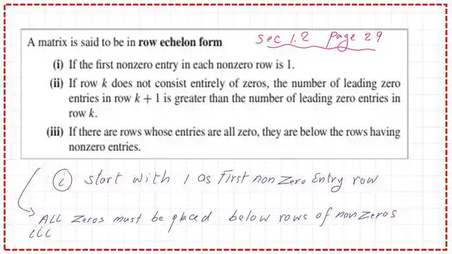
These are the three items for the REF, which stands for the free echelon form based on the leading item being nonzeros. The last row of zeros should be the bottom row.

The following slide image includes a definition of the REF.

What is the RREF (reduced row echelon form)?
The RREF stands for the reduced-row echelon form. This form includes the three previous items included in the RE form, but all leading entries must be 1s.
The column that has the first leading one should have zeros below it. At the same time, the columns of the leading ones should include zeros above and below the leading ones.

This is the case of a 3×3 matrix in the REF. We have a diagonal matrix with three ones; the leading items are nonzero. The first leading one has two zeros below the leading item.

This is the case of a 3×4 matrix in augmented form. We have a diagonal of non-zero items, shown as ones. The solid boxes include any possible values.
The pivot column in matrix A corresponds to the leading items. In the shown matrix, there are three leading ones, indicating three pivot columns.

The use of the RREF to solve a system of linear equations.
The RREF echelon form is the method Gauss-Jordan uses to obtain the solution to linear equations, avoiding the back-substitution method.
Step 1: Create an RE form using row operations.
Step 2: Use the leading term in the third row to create a zero for the elements above it.
Step 3: Use the second row’s leading term to create a zero for the element above it.
Based on these operations, the values in the fourth column will change, and at the end, we can obtain the values of the unknowns directly.
For instance, if we have the following system of linear equations: x+y+z=6 & 2x-y+z=5 and 3x+y-2z=9.
Perform a row operation to create an RREF, and we will get the arranged augmented matrix.
This new arrangement will give us the values x = 3, y = 2, and z = 1. There is no need to use the back substitution to get these values.

Another example of the Reduced Echelon form.
In the given matrix A, which has a dimension of 4×5, row reduction must be performed to locate the pivot columns.
The first row has a leading term of zero, which cannot be accepted, so we will replace it with row number 4, which has a leading term of 1 and is accepted as a non-zero item.
We will perform a series of row operations to make the items below the first leading item zeros. These steps create the reduced echelon form for a 4×5 matrix. The shape of the reduced echelon form is shown in the next slide image.

We have the third row containing five zeros, which we cannot accept, and we will swap the third row to the fourth row to match the condition of the REF. The places of the leading items and the pivot columns are shown in the next slide image. the leading terms are 1& 2& -5 which are a11 & a22 and a34.

We have used the REF to identify the positions of the leading terms and the pivot column, so we will return to the original matrix A with this information in the next slide image.

The pdf data for this post can be viewed or downloaded via the next document.
In the next post, we will look at practice problems for back substitution.
This is a link to the matrix calculator.
For a useful external link, math is fun for the matrix part.