Last Updated on March 6, 2026 by Maged kamel
- Solved problem 6-8 for local buckling of columns-CM#14.
- Detailed descriptions of problems 6-8 on local buckling.
- Properties of the HSS section from Table 1-11.
- Check whether the HSS section is long or inelastic.
- Find Fe and check whether the HSS section is slender or non-slender.
- Estimate Be and he for the HSS section.
- Estimate the value of the reduction factor Q.
- Estimate the factored design nominal strength values.
Solved problem 6-8 for local buckling of columns-CM#14.
Description of data.
The following slide image contains a brief description of the content of this post.
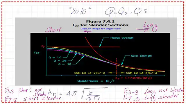
The slide before you contains the shapes for various Q values, the Euler graph, and the limiting vertical line for the short and long columns. The formula for local buckling of columns is included.
Our Fcr value, when Kl/r>4.71*sqrt(E/Q*Fy), Fcr=0.877* Fe. Our Fcr value, when Kl/r>4.71*sqrt(E/Q*Fy), Fcr=0.877* Fe.
The yellow curve at the left side of the vertical line, for the case of kl/r<=4.71*sqrt(E/Q*Fy), when Qfy/fcr<=2.25, then the fcr=Q(0.658^QFy/Fe)*QFy, and the different value of Qs, from A beginner’s guide to the steel construction manual, and the shapes of the graph accordingly.
From the next slide, we have Chapter E for the design of members for compression. Part E3 for short and long columns and the table note E1.1, selection table for the application of Chapter E sections.
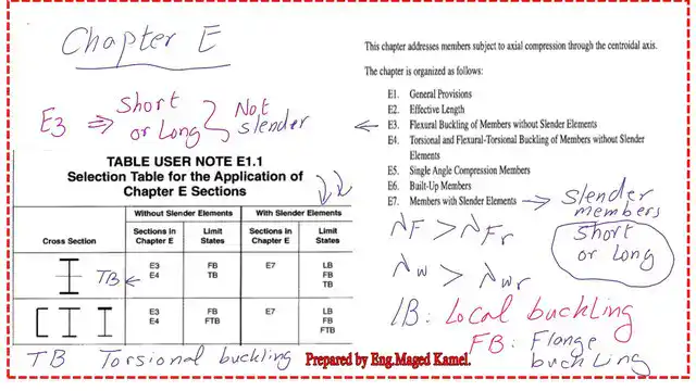
For the W-section, without slender elements, in sections in chapters E3 and E4’s limit state, Fb stands for flexural buckling and Tb for torsional buckling.
In the case of slender elements, when λf>λr, where λf = flange b/t, λw = web b/t>λrw, E7 will control the design and relevant parameters. All elements are for flexural and torsional buckling.
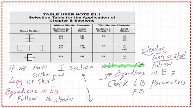
The third item in the following table is the section for the tube section, E3, without the slender section. When λ<λr, it is a stiffened section, and when λ >λr.
Then, E7 will address slender elements for the limit states of local buckling and flexural buckling.
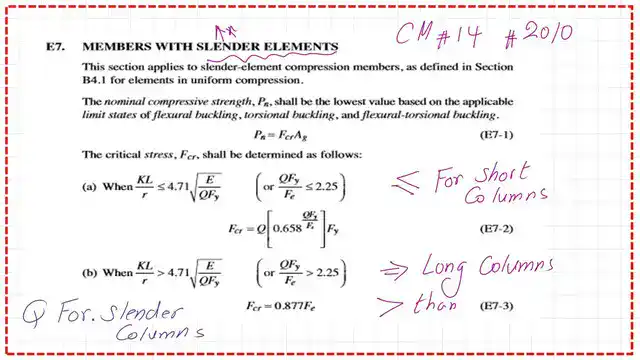
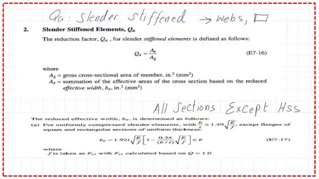
This is part E7: members with slender elements; the coefficient for the short and long columns for items E7-1 to E7-3. The Q=net reduction factor accounts for slender compression elements, Q=Qs*Qa, when our λ>λr for the flange and web.
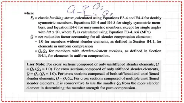
For a cross-section composed of only unstiffened slender elements, since Q=Qs*Qa, since Qa for unstiffened elements is 1, then Q=QS. For an angle, the section is unstiffened.
For cross-sections composed of only stiffened elements, َQ=Qs*Qa, Qs=1, for the case of a tube, then Q=Qa.
For the general condition for Q=Qa*Qs, sections comprise multiple unstiffened slender elements.
It is conservative to use smaller Qs from the more slender elements to determine the member strength on the next slide; for slender stiffened elements, the parameters for Qa and be are the reduced effective breadth.
The following slide image contains Table B4.1A for compression members for unstiffened elements.
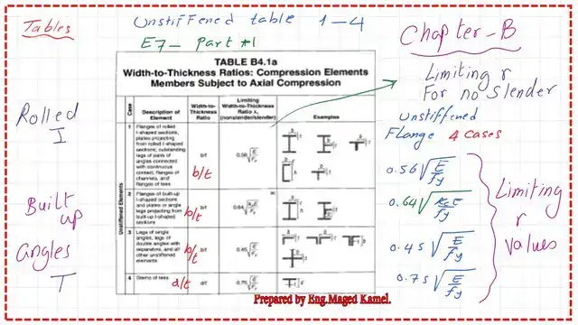
The following slide image contains Table B4.1A for compression members for stiffened elements.

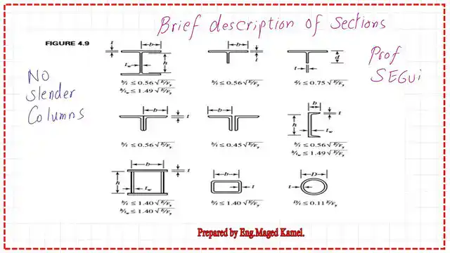
This is a brief description of sections that are not slender for compression members, from Prof. Segui’s handbook, with slenderness ratios included for each shape.
The data for section E7 clause is shown on the next slide, and the different values of critical stress Fcr.
What are the items Qs, Qa, and Qs?
How can we find Qa and be values?
Detailed descriptions of problems 6-8 on local buckling.
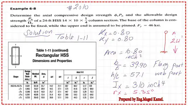
For the solved problem 6-8, determine the axial compressive design strength Φc Pn and the allowable design strength Pn/λc of a 24 ft HSS of 14x10x1/4 inch column section; the base of the column is considered to be fixed.
The upper end is assumed to be pinned. Fy=46 ksi. The effective length factor k for the column is 0.7, but the recommended value is 0.8. Refer to table C-A-7.1 of the specification.
Properties of the HSS section from Table 1-11.
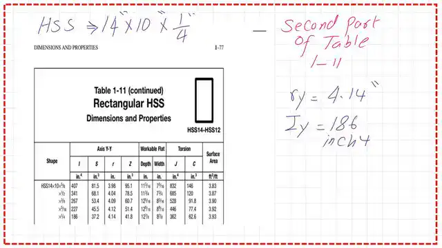
Use Table 11-11, parts 1 and 2, for detailed properties. We will get a design section of 0.233-inch wall section, the area is 10.80 inch2, b/t =39.9, h/t=57.1, Ix=310 inch4, rx=5.35 inch2, Iy=186 inch4, ry=4.14 inch2 from part 2.
This is part 2 of Table 1-11, from which we get the values of ry and Iy: ry = 4.14 inches and Iy = 186 inch4.
Check whether the HSS section is long or inelastic.
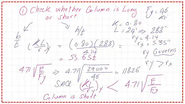
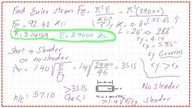
The next step is to check whether the column is inelastic or long; the limiting ratio is 4.71*sqrt(E/fy )= 4.71*sqrt(29000/46)=118.26.
To compare this value to the K*L/r at the y-direction, Kl/r at y=0.8*24*12/ 4.14 =55.652. This is the maximum value as compared to Kl/r y since rx> ry.
The kl/r at y= 55.652 compared to 118.26. Since kL/r at y < 118.26, the column is short; proceed to find the Euler strength, which will be =92.42 ksi, as shown in the figure.
Find Fe and check whether the HSS section is slender or non-slender.
We estimate the Euler stress based on the given section. To determine whether the HSS section is slender, we check the B/t value against the limiting value for the slenderness ratio for a stiffened HSS section. The section is slender since b/t is bigger than 35.15. Please refer to the next slide image for more details.
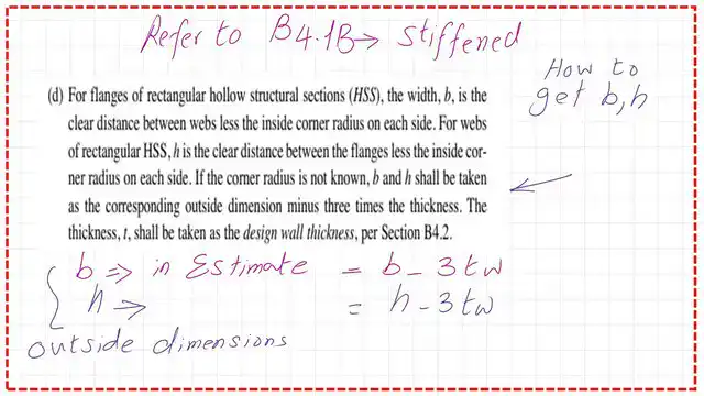
Based on B4.1b for stiffened elements, it is recommended to calculate a modified b=b-3*td and modified h to be equal to h-3td where t design equals 0.233 inches, h=14 inches, and b=10 inches.
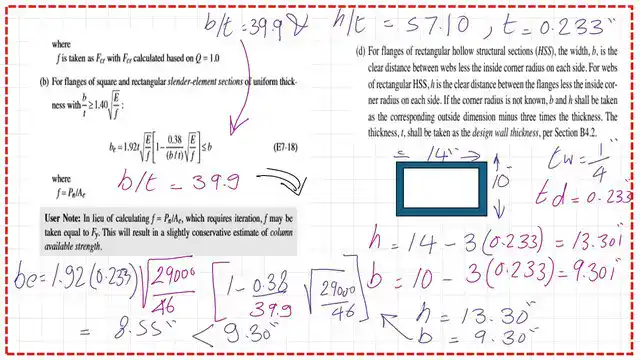
Estimate Be and he for the HSS section.
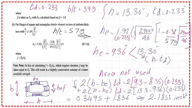
The value of b=10-3*(0.233) =9.301 inch, while h =14-3*(0.233)=13.301. We estimate the values of be and he as follows: be =1.921*ts*sqrt(E/Fy)*(1-0.38/b/t*sqrt(E/Fy)).
Please have a look at the following slide for more details on the value of b for the smaller HSS section width.
Please have a look at the following slide for more details on the value of the HSS section’s larger width. The value of the deducted area is shown.
Estimate the value of the reduction factor Q.
Since the column is short, we divide the effective area by the gross area to get the Q value.
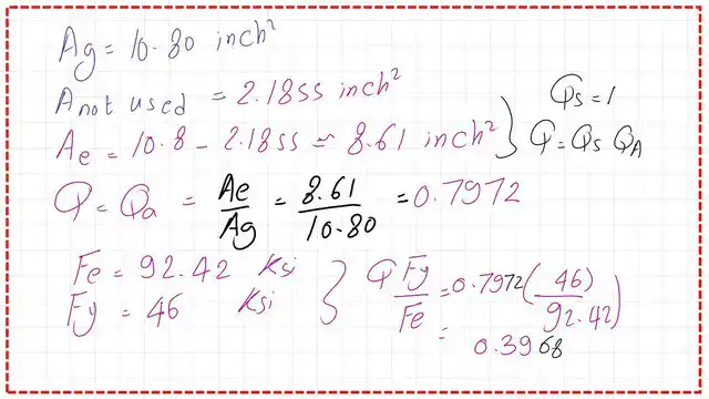
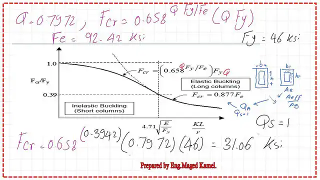
Estimate the critical stress for the HSS section. For the Fcr calculation, Fcr =(Q*fy)*0.658^(Qfy/fe), since Q=0.7972, fcr (0.7976*46)*(0.658)^(0.7976*46/92.49), Our fe=92.42 ksi.
Estimate the factored design nominal strength values.
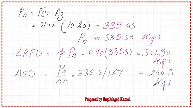
Then the nominal load Pn=Ag*fcr=10.8*31.05=335.45 kips.
For the available strength LRFD, Φc=0.90, ΦcPn=0.9*335.45=301.9 kips.
For the ASD, Pn/Ωc = 335.30/1.67 = 200.90 kips.
This solved problem discussed the idea that a section is reduced when a hollow section is treated as a stiffened element due to local buckling. By becoming smaller, only be, he is functioning; the effective area can be estimated and called Aef.
The Qa can be estimated as Aef/Ag. Then, add this Q value to the graph to get Fcr.
This is the PDF file for this post.
If you have the link, refer to theprevious post: A Solved problem 5-3 for local buckling of columns.
The following post: A solved problem 6-19-4.
For a good A Beginner’s Guide to the Steel Construction Manual, 14th ed. Chapter 7 – Concentrically Loaded Compression Members.
For a good A Beginner’s Guide to the Steel Construction Manual, 15th ed. Chapter 7 – Concentrically Loaded Compression Members.
For a good A Beginner’s Guide to the Steel Construction Manual, 16th ed. Chapter 7 – Concentrically Loaded Compression Members.
.