Last Updated on January 12, 2026 by Maged kamel
How to Use a Matrix for the Quadratic Function?
We discussed the quadratic function, or quadratic interpolation function, in two posts. The first post provides an easy introduction to quadratic interpolation, and the second post solves problems using it.
Understanding the matrix representation of quadratic functions is essential for solving quadratic equations efficiently.
The matrix for the quadratic helps determine the quadratic function’s coefficients accurately.
In this post, we will solve three problems. The main idea behind these practice problems is to use the matrix of a quadratic function to determine its parameters, or, more simply, to obtain the quadratic matrix.
The first practice problem for the matrix of the interpolating polynomial function
Use row echelon form to obtain the a0, a1, and a2 values.
We need to find the interpolating polynomial P(t) = a0 + a1t + a2t2 for the given data points (1, 12), (2, 15), and (3, 16).
We start by writing the three equations for P(t) for the given three points as follows:
To illustrate, we will demonstrate the process using the quadratic function matrix to solve specific problems.
We plug in the value of t=1, and P(1) equals 12. The first equation is P(1)=a0+a1(1)+a2(1)^2=12. We plug in the value of t=2, and P(1) equals 15. The second equation is P(2)=a0+a1(2)+a2(2)^2=15. We plug in t = 3, and P(1) equals 16. The second equation is P(3)=a0+a1(3)+a2(3)^2=16.
Our unknowns are a0, a1, and a2. Using the augmented matrix, we will find the first row as (1 1 1 12), the second row as (1 2 4 15), and the last row as (1 3 9 16). We will convert the augmented matrix to the row echelon form.
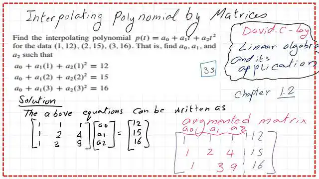
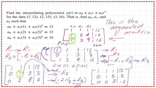
The first row has a leading item equal to 1; to set a21 and a32 to 0, we will perform the elementary row operations, as shown in the next slide.
We will multiply the first row by -1 and add the value to the second row, and for the third row, we will multiply the first row by -1 and add the value to the third row.
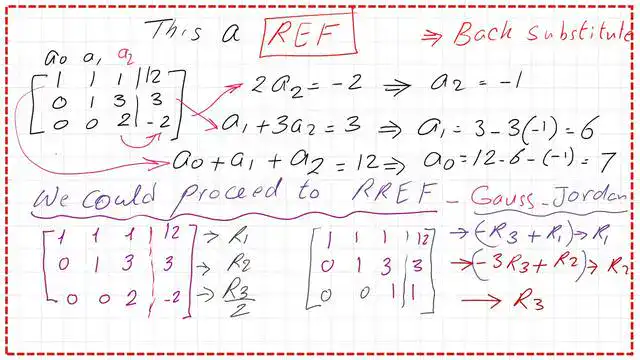
Next, we will move to the second-leading item in the second row, which is 1; we will let a22 equal 0 by multiplying the second row by -2 and adding the result to the third row. As we can see, the quadratic function is in row echelon form. We have a0=7. We can use back-substitution to find the values of a1 and a2.
Using the matrix for the quadratic function simplifies the equation-solving process.
By using the quadratic matrix, one can quickly analyze relationships between variables.
Use a reduced row echelon form-interpolating polynomial function.
If we wish to use the reduced row echelon form for the matrix of the quadratic function, we want zeros above the pivots in the third and second rows. We consider a33 as a pivot, then multiply R2 by -3 and add the result to R2; we will get a zero in the a23 element. We will multiply the third row by -1 and add the value to the first row.
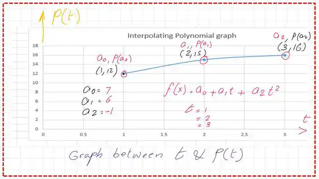
Next, we will move to the second pivot column. Multiply R2*-1 and add the value to R4; we will get a zero for element a12. We have a0=7, a1=6, and a2=-1. We can rewrite the interpolating polynomial as P(t)= 1+6*t-t2.
Using the matrix for the quadratic efficiently helps visualize the solution process.
The second practice problem emphasizes the practical use of the matrix for the quadratic polynomial function.

Using the quadratic matrix provides a framework for determining the function’s behavior.
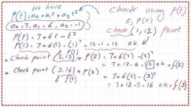
Check the interpolating function for the three points given. The details of the value of t and the corresponding value of f(t) are in the next slide image.
This is a graph for the interpolating Quadratic polynomial.
The second practice problem for the matrix of the quadratic polynomial function.
The second practice problem is a matrix problem for the quadratic polynomial function. It is required to find the quadratic polynomial function P(t)=a0+a1x+a2x^2 that satisfies the condition P(0)=f(0), p'(0)=f'(0) and p”(0)=f”(0).
In this practice problem, instead of giving three points. One point is given, and the slope at that point shall equal the slope of the original function, e^2x. The second derivative P”(0) is also equal to the second derivative of the original function, which is e^2x.
The interpolating quadratic polynomial y value at point zero is estimated by plugging in the function e^2x and setting x=0; the value at point zero equals e^0=1.
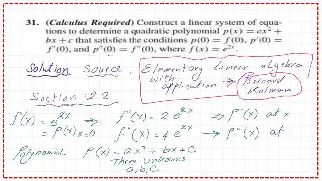
The three polynomial equations are written in terms of x. Please refer to the next slide image.
The insights from the quadratic matrix are invaluable for understanding polynomial functions.
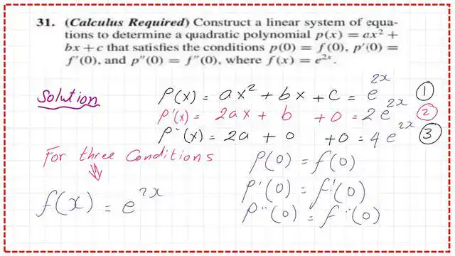
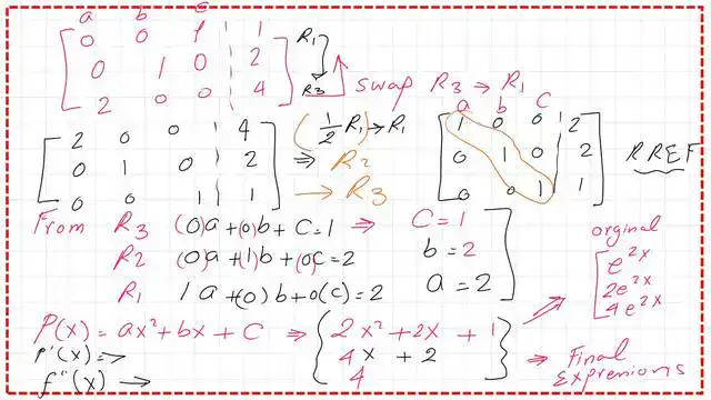
The first and second derivatives of the original function are estimated at x=0, as shown in the next slide image. We start by writing the three equations for P(x) for the given data. We plug in x=0, and P(0)=1.
The expression is P(x)=ax^2+bx+c. The first equation is P(0)=a(0)^2+b(0)+C=1. We plug in the value of P'(0), equal to 2. The expression is P'(x)=2ax+b. The second equation is P'(0)=2a(0)+b=2.
We plug in the value of P”(0), equal to 4. The expression is P”(x)=2a. The third equation is P”(0)=2a=4. We can write the three equations in the form of two-matrix multiplication. The product is equal to (1 2 4).
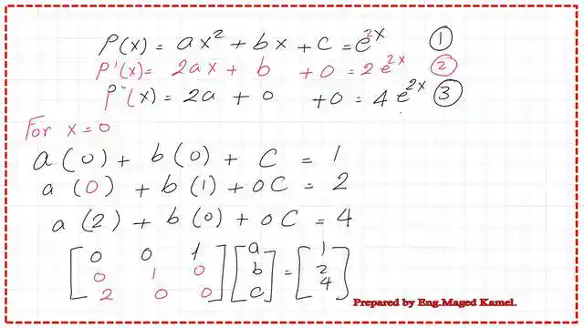
We can write the augmented matrix. We will swap the first and third rows in the row echelon form and convert it to a reduced echelon form. The final values for a, b, and c are a = 2, b = 2, and c = 1.
The final polynomial generated from the quadratic function’s matrix provides a clear representation of the data.
This problem demonstrates how the quadratic function’s matrix can be applied in real-world scenarios.
The polynomial can be written as p(x) = 2x^2 + 2x + 1.
The following slide image shows the derivatives of the polynomial function and the original functions.
The matrix for the quadratic serves as a crucial tool in theoretical and applied mathematics.
By applying the quadratic matrix, we obtain a more accurate analysis of the function.
In conclusion, mastering the quadratic matrix is key to advancing in polynomial analysis.
The third practice problem for the quadratic polynomial function.
For the third practice problem for a quadratic matrix.It is required to find the quadratic polynomial function P(t)=a0+a1x+a2x^2 that satisfies the condition P(1)=f(1),p'(1)=f'(1) and p”(1)=f”(1).
One point is given, and the slope at that point shall equal the slope of the original function, which is xe^(x-1). The second derivative P”(0) is also equal to the second derivative of the original function, which is xe^(x-1). The interpolating quadratic polynomial y value at point zero is estimated by plugging in the function xe^(x-1) and setting x=1; the value at point zero equals 1*e^(1-1)=1.
The first and second derivatives of the original function are estimated at x=1. The next slide image shows how to estimate these values.
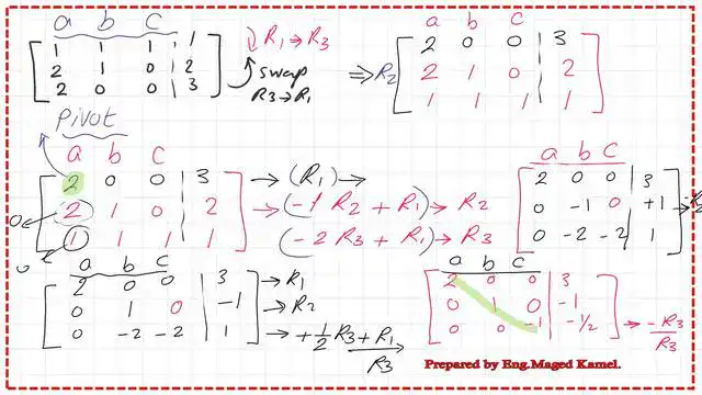
We start by writing the three equations for P(x) for the given data.
We plug in x=1, and P(1)=1. The expression is P(x)=ax^2+bx+c.The first equation is P(1)=a(1)^2+b(1)+C=1. We plug in the value of P'(1), equal to 2. The expression is P'(x)=2ax+b.
The second equation is P'(1)=2a(1)+b=2. We plug in the value of P”(1), equal to 3. The expression is P”(x)=2a. The third equation is P”(1)=2a=3.
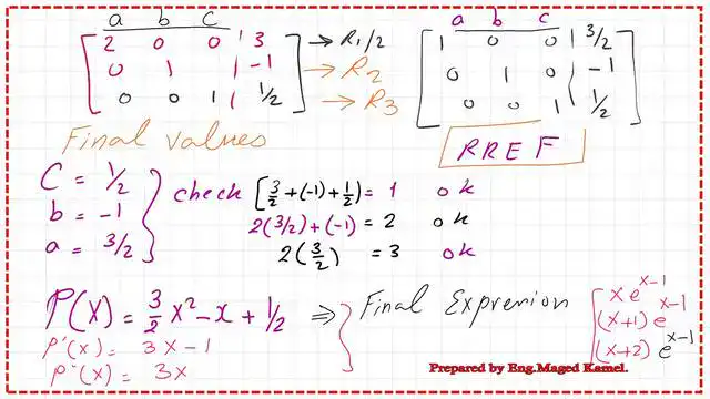
We can write the augmented matrix. We will swap the first and third rows in the row echelon form. We have a row echelon form for the third practice problem. We will convert it to the reduced echelon form.
For further reading on the matrix for the quadratic, visit math is fun.
We can write the augmented matrix. We will swap the first and third rows in the row echelon form and convert it to a reduced echelon form.

The final values for a, b, and c are a = 3/2, b = -1, and c = 1/2. The final value of the polynomial is shown in the next slide. The following slide image shows the derivatives of the polynomial function and the original functions.

The pdf data for this post can be viewed or downloaded via the next document.
For a useful external link, math is fun for the matrix part.