
Last Updated on November 1, 2026 by Maged kamel
Gauss Elimination with Complete Pivoting- 2×2 Matrix
This Post demonstrates why complete pivoting is necessary when solving a 2×2 linear system with Gaussian elimination using four-digit arithmetic and rounding. Direct elimination with the very small pivot 0.003 produces a huge multiplier, significant rounding errors, and an incorrect solution. This Problem is taken from Numerical Analysis by Richard Burden.

Video for the solved Problem with complete Pivoting: A Complete Guide- 2×2 Matrix
The following video illustrates this Post’s content.
Timestamps for Video:
- 00:00 Introduction to complete pivoting for a 2×2 Matrix.
- 00:42 A solved Problem #2.00. 01:52 Find the absolute maximum Value for a11 and a21.
- 02:23 Find the absolute maximum Value for a21 and a22.
- 03:31 Swap the 2nd column with the first column.
- 05:12 Determine the Value of m21.
- 06:00 What are the values of the elements a21, a22, and b22?
- 07:52 The final Value for x2′. 08:15 The final Value for x1′
- 09:00 The final values for x1 and x2.
- 09:32 The complete pivoting technique data by the author.
Step 1: Find the maximum absolute Value for the first Row.
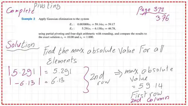
First, the equations are: 0.003×1 + 59.14×2 = 59.17, and the Second equation is 5.291×1 – 6.130×2 = 46.78. We will follow a new technique called complete pivoting; we evaluate the maximum absolute Value for all elements.
We will check the maximum absolute Value for the first Row. For the first Row, the maximum absolute Value is the maximum absolute Value of (0.003 and 59.14); this gives 59.4 for the first Row.

For the Second Row, the absolute maximum of 5.29 and 6.13 is 6.13. Then the maximum absolute Value of (59.14, 6.13) is 59.14, which is the element in the first Row, Second column. Please review the following slide.
Step 2: Swap the Second column with the first column.
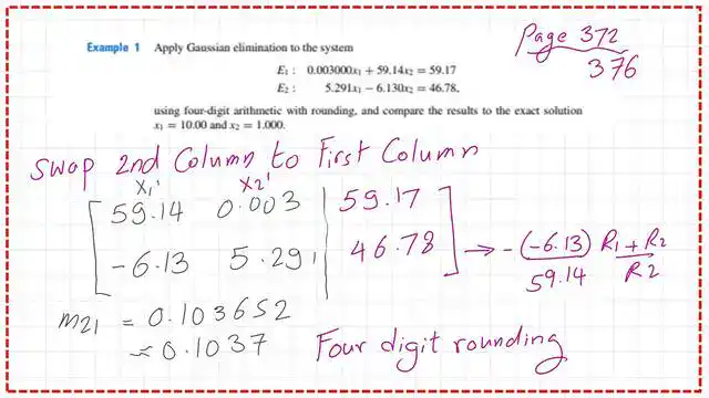
We swap the Second column to become the new first column, and the old first column will be the new Second column.
The following slide shows the elements after we swap the Second column; the variables become x1′ and x2′. The new augmented maMatrixill be 59.14 then 0003, and the right-hand side is 59.17; for the next new Second Row, it will become -6.13, .291, and the right-hand side is 46.78.
We will estimate -m21, the multiplier, which equals -(-6.13/59.14)=0.103652; rounded to four digits, it is 0.1037; we will multiply by the first Row and add the result to the Second Row.
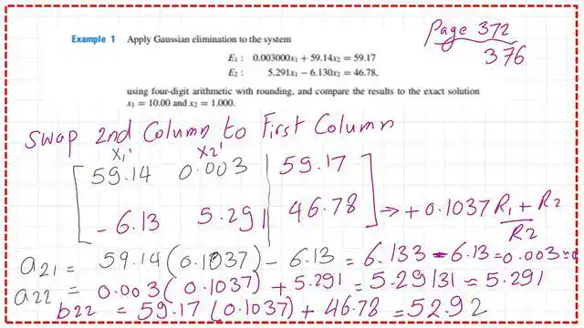
Use a11 as the pivot; the new Value of a11 will be 0.003*59.14-7.13=0.003, assuming a=0.
For a22, the new Value of a22 will be 0.003*0.1037+5.291=5.291.
For b22, the new Value of b22 will be 59.17*0.1037+46.78=52.92.
Step 3: What are the values for x1 nd x2?
So for x2 dash, we are going to divide 52.92 by 5.291= 10.002, rounded to 10. We substitute back to find the Value of x1 dash.
The x1 dash Value is (59.17-0.003*10) divided by 59.14=1.0. Please refer to the following slide for more details.
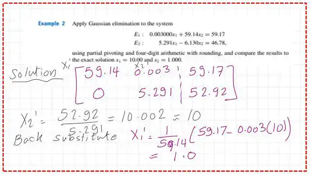
Again, we know that x1 dash equals x2 in reality 2; the final Value of x2 will be 1, and x2 is in reality x1.
As you can see, these two values match the exact solution for x1 and x2 on the last slide.

This is the complete pivoting from the author, page 379. Pivoting can involve interchanging both rows and columns, as we did. We checked the maximum absolute values in Row 1 and Row 2, and we found that a12 is the largest Value among a11, a21, and a22.

You can view and download the PDF for the solved Problem from this Link.
Link to the Previous Posts: 13-Gauss Elimination with Partial Pivoting: 2×2 Matrix
For scaled pivoting, refer to Post 14- 14-Gauss Elimination with Scaled Pivoting: 2×2 Matrix.
This is the Omni calculator for estimating various linear algebra items: LU Decomposition Calculator.
Link to the the Omni calculator:: LU Decomposition Calculator.
Another calculator to use is the Matrix Calculator.