40- Easy Design of steel section for continuous beam-4-4

Solved problem 10-1 for the Design Of Steel Section For Continuous Beam-Part-4/4.

The negative moments are due to dead uniform loads and concentrated loads.

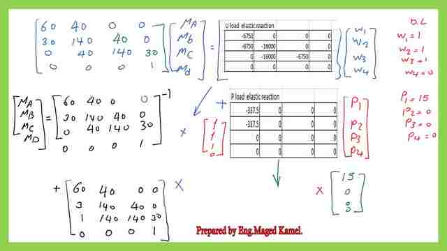
We will substitute the values of spans and loads; the general form of the matrix, as we have done, enables us to use the form to get the values of the bending moments for different span lengths and different values of loadings.

The values of span lengths are for the first span length L1=30′, for the second span length L2=40′, and for the third span length L3=30′.

We will substitute in the first matrix,as 2*L1=60, L2=40′ , L1=30′ 2*(L1+L2)=2*(30+40)2*70=140′, 2*(L21+L3)=2*(40+30)2*70=140′, we will put the zeros where it is located in the matrix.

As for the elastic reactions matrix for the uniform loads vector matrix, we have -L1^3/4=-(30^3/4)& -L2^3/4=-(40)^3/4 &-L3^3/4=-*(30)^3/4.

As for the elastic reactions matrix for the concentrated load’s vector matrix, we have only one parameter, which is -(3/8)*L1^2=-(3/8)*(30)^2, which we will substitute in the next slide. These are the values as shown for the matrix 4×4, which is the vector-matrix for moments (MA MB MC MD).

I have used an excel sheet to solve, and these are the values for the elastic reaction parameters for the vector matrix for uniform loads. These are the original parameters as shown, -L1^3/4=-(30)^3/4=-6750& -L2^3/4=-(40)^3/4=-16000& -L3^3/4=-(30)^3/4=-6750.

These are the corresponding values after substitution for the uniform load matrix, also these are the related values after substitution for the concentrated load matrix.

The dead load value W1=1 kips/ft, which is the dead load value for all the spans, while W4=0. P1 value=15 kips, which is the dead load for the first span. P2=P3=P4=0, since no concentrated loads for the second and third spans.

We need to estimate the inverse of the matrix to solve for the values of the negative moments we can get the inverse value of the matrix by using excel or other programs, and the matrix inverse is denoted by the symbol -1.

When multiplying by the inverse matrix, on the left-hand side, we get the unity matrix, where the diagonal is 1 and all other elements are zeros.

This is the inverse of the matrix that will be multiplied by the elastic reaction coefficient and by the column-vector uniform load matrix, which is (1 1 1  0), this is the part for the moment values due to the uniform loads, while for the moment values due to the concentrated loads.

We will multiply the inverse of the matrix by the elastic reaction parameters, again by the concentrated load’s column-vector matrix. Where P1=15 kips, P2=P3=P4=0, the vector column matrix is( 15 0 0 0). We have the vector column matrix on the left-hand side with (MA MB MC MD) and two matrices added together.

For the moment values from the uniform loads plus the moment values from the concentrated loads. We can find out the values of the bending moments as shown in the next slide. MA, MB, MC, MD, the first figures are for the moments due to uniformly distributed loads plus the moments due to concentrated loads.

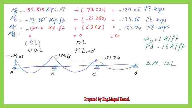
For Wd=1.0 kips/ ft and P1, dead load=15 kips/ft, this is the bending moment due to the dead loads.

The negative moments are due to live uniform loads and concentrated loads.

We can get the moment values for the live loads after substituting their values. We will see the values of the corresponding live loads which are Wl=3 kips/ft, P live load =20.0 kips the corresponding moment values are shown in the next image.

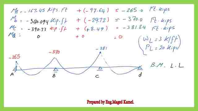
The bending moment diagram is due to Dead loads.

The B.M diagram for the Dead loads is drawn in the next slide image.

The maximum negative and positive values moments.

In the cases of loading, for the maximum negative moment, we add the Dead load plus the live loads for two neighboring spans, while for the maximum positive moment, we add the dead load plus the live loads for the alternate spans.

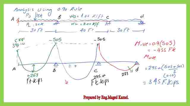
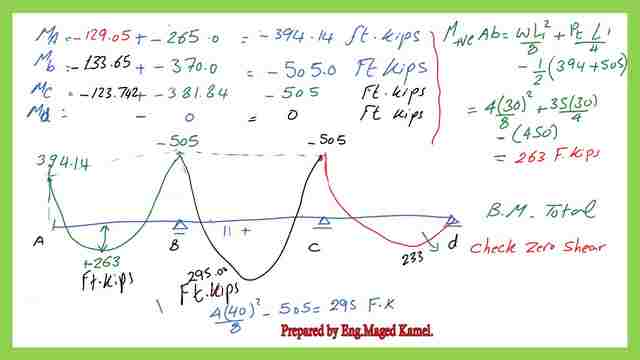
If we add both diagrams, we will get the same values as shown by Prof. Mccormacks’s textbook. The moment at the fixed support MA =394.14 Ft.kips, while the moment at support B,  MB=-505.0 Ft.kips.

The moment at support C,  MC=-505.0 Ft.kips. The moment at support D,  MD=0 Ft.kips. For the positive bending moments.

We have two values of bending moment, the first one is W*L1^2/8, where w is the w total=(wd+wl).
Wt=1+3=4 kips/ft, L1=30′, Wt*L1^2/8=4*30^2/8=450 ft.kips.

The second moment is due to the total concentrated loads Pt=Pd+Pl=15+20=35 kips. The moment due to this case is PtL1/4=3530/4=262.50 ft-kips. We will deduct the average of (394.14+505.00), which is (-449.57 Ft.kips).

The moment at the fixed support MA =394.14 Ft.kips, while the moment at support B,  MB=-505.0 Ft.kips.
The moment at support C,  MC=-505.0 Ft.kips. The moment at support D,  MD=0 Ft.kips. For the positive bending moments.
We have two values of bending moment, the first one is W*L1^2/8, where w is the w total=(wd+wl). Wt=1+3=4 kips/ft, L1=30′, Wt*L1^2/8=4*30^2/8=450 ft. kips.

The second moment is due to the total concentrated loads Pt=Pd+Pl=15+20=35 kips. The moment due to this case is Pt*L1/4=35*30/4=262.50 ft-kips. We will deduct the average of (394.14+505.00), which is (-449.57 Ft.kips).

The final value of the positive bending moment=263.0 Ft.kips for span AB.

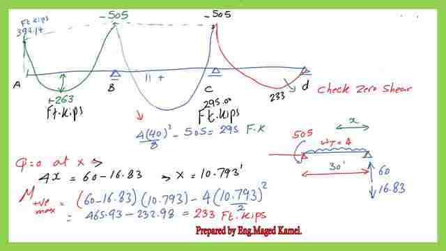
While for span BC, the final value of the positive moment=4*30^2/8-(0.50*(505+505))=295.0 Ft.kips.For the positive moment for the span CD, the maximum positive moment for the span CD is not located at the mid-span.

But that position will be at the place where the shear value=0.

From the next slide, the positive moment is assumed at X distance from the left support, where the shear value Q=0 and the reaction at D is RD.

For span length=30′, Rd=4*0.5*30-(505/30)=60-16.83=43.17 kips.

The shear at X distance=4*X-43.17=0, then X=10.793′, to get the maximum positive moment value=RD*X-Wt*L3^2/2=(43.17*10.793)(4*10.793^2/2)=233 Ft.kips as shown in the sketch and as indicated in the author’s solution.

The elastic redistribution for a moment or 0.90 rule.

For the maximum positive value of Moment, we have span AB with M+ve=+263.0 Ft.kips, we have span BC with M+ve=+295.0 Ft.kips, we have span CD with M+ve=+233.00 Ft.kips, the largest value is =+295.0 Ft.kips, we add the 0.10*average of (505.0).

The moment diagram due to the maximum negative moment is equal to 505 Ft.kips. While the maximum positive moment is 295.0 ft. kips. These values are prior to using the 0.90 rule.

The final value of positive moment =295.0 +0.10*(505)=345.0 Ft.kips. The maximum negative moment for beam =0.90*505=455 Ft.kips, which is >M positive max which is 345.0 ft. kips.

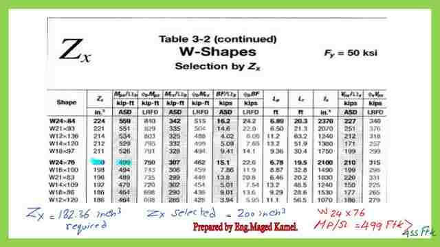
Design of steel section for continuous beam based on the maximum moment.

The Nominal moment Mn=760.0 ft.kips, convert to inch.kips=76012=9118.20 inch.kips. Since Mn=FyZx, Fy=50 ksi, then Zx=Mn/Fy=9118.20/50=182.36 inch3. we use table 3.2, to select the appropriate lightest W section. For the steel section for continuous beam, Zx required 182.36 inch3.

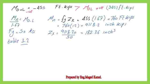
For the ASD, we have MT= 455 Ft.kips, for the nominal moment, we have Ω=Mn/Mt=1.67, then Mn=1.67*455=760.0 ft. kips,  but if we have solved using 1.20D+1.6L then Mn=Mult*(1/Φb).Φ=0.90, Mn=1.11*Mult.

The selected Zx is W24x76 which has Zx=200.0 inch3. Mpx/Ωb =499.0 ft. kips > 455.0 ft. kips. This is the Final check for the design of the steel section for continuous beam 3-3.

This is a link to the previous post.

This is the pdf file used in the illustration of this post.
Have more information about the structural analysis –III.
For more details about the upper bound and lower bound